Markov Decision Process

A Markov decision process is a $5$-tuple $(S,A,P_{\cdot}(\cdot,\cdot),R_{\cdot}(\cdot,\cdot),\gamma)$, where

$S$ is a finite set of states.
$A$ is a finite set of actions (alternatively, $A(s)$ is the finite set of actions available from state $s$).
$R_{a}(s,s’)$ is the immediate reward (or expected immediate reward) received after transitioning from state $s$ to state $s’$, due to $a$. It can also be like $R(s)$ or $R(s,a)$.
$P_a(s,s’)=P(s_{t+1}=s’|s_t=s,a_t=a)$ is the probability that action $a$ in state $s$ at time $t$ will lead to state $s’$ at time $t+1$.
$\gamma\in[0,1]$ is a discount factor, which represents the difference in importance between future rewards and present rewards.

The solution to the MDP is the policy $\pi(s)\rightarrow a$, which maximizes the long-term expected reward. In reinforcement learning domains, we simply assume the policy is deterministic and history-independent.

Total Reward

$V(s)$, the state value function, is the total discounted reward from time-step $t$,

$\begin{align*}V(s_t)&=R(s_t)+\gamma R(s_{t+1})+\cdots\\ \qquad\qquad&=\sum\limits_{i=t}^{\infty}\gamma^iR(s_{i})\qquad 0\leqslant\gamma\leqslant 1 \end{align*}$

We can show that

$V<\infty$

Policies

$\begin{align*}\pi^*&=\mathop{\arg\max}_{\pi}\mathbb{E}V^{\pi}\\ &=\mathop{\arg\max}_{a}\sum\limits_{s'\in S}P_a(s,s')V(s') \end{align*}$

The long term and delayed reward is given by

$V^{\pi}(s)=\mathbb{E}[V(s_0)|\pi,s_0=s]$

which is not equal to the immediate reward $R(s)$.

From Bellman Equation, the value function can be decomposed into two parts:immediate reward $R(s)$ and discounted value of successor state $\gamma V(S_{t+1})$.

$\begin{align*} V(s) &=\mathbb{E}[V|S_t=s]\\ &=\mathbb{E}\left[\sum\limits_{i=0}^{\infty}\gamma^iR_{i}|S_t=s\right]\\ &=\mathbb{E}[R(s)+V(s)|S_t=s]\\ &=\mathbb{E}[R(s)+\gamma V(S_{t+1})|S_t=s]\\ &= R(s)+ \gamma\sum\limits_{s'\in S}P_a(s,s')V(s') \end{align*}$

Policy-Iterated RL

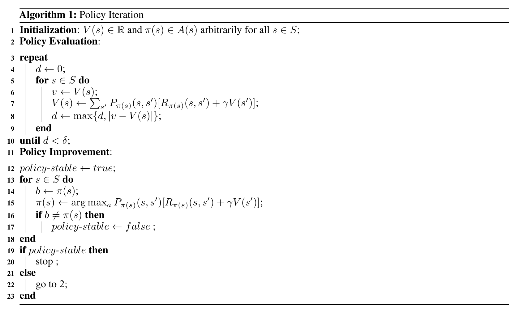
Policy iteration tries to evaluate and improve the policy in turn. Once a policy $\pi$ has been improved by using $V^{\pi}$ to yield a better policy $\pi’$, we can then compute $V^{\pi’}$ and improve it again to yield an even better policy. We can thus obtain a sequence of monotonically improving policies and value functions: $\pi_0\xrightarrow{E}V^{\pi_0}\xrightarrow{I}\pi_1\xrightarrow{E}\cdots \xrightarrow{I}V^{\pi^{\ast}}\xrightarrow{E}V^{\ast}$
where $\xrightarrow{E}$ denotes a policy evaluation and $\xrightarrow{I}$ denotes a policy improvement. Each policy is guaranteed to be a strict improvement over the previous one (unless it is already optimal). Because a finite MDP has only a finite number of policies, this process must converge to an optimal policy and optimal value function in a finite number of iterations.

Value-Iterated RL

One drawback to policy iteration is that each of its iterations involves policy evaluation, which may itself be a protracted iterative computation requiring multiple sweeps through the state set. If policy evaluation is done iteratively, then convergence exactly to occurs only in the limit.

In fact, the policy evaluation step of policy iteration can be truncated in several ways without losing the convergence guarantees of policy iteration. One important special case is when policy evaluation is stopped after just one sweep (one backup of each state). This algorithm is called value iteration. It can be written as a particularly simple backup operation that combines the policy improvement and truncated policy evaluation steps:

$\begin{align*}V_{k+1}(s)&=\max\limits_a \mathbb{E}[ r_{t+1}+\gamma V_k(s_{t+1})]|s_t=s, a_t=a)\\ &=\max\limits_a \sum\limits_{s'} P_a(s,s')[ R_{a}(s,s')+\gamma V_k(s')] \end{align*}$

for all $s\in S$. For arbitrary $V_0$, the sequence $\{V_k\}$ can be shown to converge to $V^\ast$ under the $V^\ast$.

Code Example

1
2
3

import numpy as np
import gym
from gym import wrappers

Policy-Iterated RL

def policy_evaluation(env, policy, gamma=1.0):
    """ Iteratively evaluate the value-function under policy.
    Alternatively, we could formulate a set of linear equations in iterms of v[s] 
    and solve them to find the value function.
    """
    v = np.zeros(env.nS)
    eps = 1e-10
    while True:
        prev_v = np.copy(v)
        for s in range(env.nS):
            policy_a = policy[s]
            v[s] = sum([p * (r + gamma * prev_v[s_]) for p, s_, r, _ in env.P[s][policy_a]])
        if (np.sum((np.fabs(prev_v - v))) <= eps):
            # value converged
            break
    return v

def policy_improvement(v, gamma = 1.0):
    """ Extract the policy given a value-function """
    policy = np.zeros(env.nS)
    for s in range(env.nS):
        q_sa = np.zeros(env.nA)
        for a in range(env.nA):
            q_sa[a] = sum([p * (r + gamma * v[s_]) for p, s_, r, _ in  env.P[s][a]])
        policy[s] = np.argmax(q_sa)
    return policy

def policy_iteration(env, gamma = 1.0):
    """ Policy-Iteration algorithm """
    # initialize a random policy
    policy = np.random.choice(env.nA, size=(env.nS))
    # parameter
    max_iterations = 200000
    gamma = 1.0
    # run iterations
    for i in range(max_iterations):
        # calculate the value given the old policy
        old_policy_v = policy_evaluation(env, policy, gamma)
        # find the new policy
        new_policy = policy_improvement(old_policy_v, gamma)
        if (np.all(policy == new_policy)):
            print ('Policy-Iteration converged at step %d.' %(i+1))
            break
        policy = new_policy
    return policy

Evaluation

def run_episode(env, policy, gamma = 1.0, render = False):
    """ Runs an episode and return the total reward """
    obs = env.reset()
    total_reward = 0
    step_idx = 0
    while True:
        if render:
            env.render()
        obs, reward, done , _ = env.step(int(policy[obs]))
        total_reward += (gamma ** step_idx * reward)
        step_idx += 1
        if done:
            break
    return total_reward

def evaluate_policy(env, policy, gamma = 1.0, n = 100, render = False):
    scores = [run_episode(env, policy, gamma, render) for _ in range(n)]
    return np.mean(scores)

env_name  = 'FrozenLake8x8-v0'
env = gym.make(env_name).unwrapped
optimal_policy = policy_iteration(env, gamma = 1.0)
scores = evaluate_policy(env, optimal_policy, gamma = 1.0, render = False)
print('Average scores = ', np.mean(scores))
# Policy-Iteration converged at step 13.
# Average scores =  1.0

Value-Iterated RL

def extract_policy(v, gamma = 1.0):
    """ Extract the policy given a value-function """
    policy = np.zeros(env.nS)
    for s in range(env.nS):
        q_sa = np.zeros(env.action_space.n)
        for a in range(env.action_space.n):
            for next_sr in env.P[s][a]:
                # next_sr is a tuple of (probability, next state, reward, done)
                p, s_, r, _ = next_sr
                q_sa[a] += (p * (r + gamma * v[s_]))
        policy[s] = np.argmax(q_sa)
    return policy


def value_iteration(env, gamma = 1.0):
    """ Value-iteration algorithm """
    v = np.zeros(env.nS)  # initialize value-function
    max_iterations = 100000
    eps = 1e-20
    for i in range(max_iterations):
        prev_v = np.copy(v)
        for s in range(env.nS):
            q_sa = [sum([p*(r + prev_v[s_]) for p, s_, r, _ in env.P[s][a]]) for a in range(env.nA)]
            v[s] = max(q_sa)
        if (np.sum(np.fabs(prev_v - v)) <= eps):
            print ('Value-iteration converged at iteration# %d.' %(i+1))
            break
    return v

Evaluation

def run_episode(env, policy, gamma = 1.0, render = False):
    """ Evaluates policy by using it to run an episode and finding its
    total reward.
    args:
    env: gym environment.
    policy: the policy to be used.
    gamma: discount factor.
    render: boolean to turn rendering on/off.
    returns:
    total reward: real value of the total reward recieved by agent under policy.
    """
    obs = env.reset()
    total_reward = 0
    step_idx = 0
    while True:
        if render:
            env.render()
        obs, reward, done , _ = env.step(int(policy[obs]))
        total_reward += (gamma ** step_idx * reward)
        step_idx += 1
        if done:
            break
    return total_reward


def evaluate_policy(env, policy, gamma = 1.0,  n = 100):
    """ Evaluates a policy by running it n times.
    returns:
    average total reward
    """
    scores = [
            run_episode(env, policy, gamma = gamma, render = False)
            for _ in range(n)]
    return np.mean(scores)

env_name  = 'FrozenLake8x8-v0'
gamma = 1.0
env = gym.make(env_name).unwrapped
optimal_v = value_iteration(env, gamma);
policy = extract_policy(optimal_v, gamma)
policy_score = evaluate_policy(env, policy, gamma, n=1000)
print('Policy average score = ', policy_score)

# Value-iteration converged at iteration# 2357.
# Policy average score =  1.0

References

Policy Iteration