Statistics

Computer Science

Logic

Set Theory

Graph Theory

Graph

• Definition
  A graph $G$ consists of a finite collection of vertices $V(G)$ and edges $E(G)$ where each edge connects a distinct pair of vertices.

  • We only discuss the undirected graph, which is the simple graph (at most one edge between any two vertices) and its edges have no orientation.
  • The order of $G$ is $|V|$ and the size of $G$ is $|E|$.
  • Two vertices are adjacent vertices if they are connected by a edge.
  • The degree of a vertice is the number of adjacent vertices of it. A vertex with an odd (even) degree is an odd (even) vertice.
  • A graph is complete if every distinct pair of vertices is connected by an edge.

• Properties

  • Graphs $F$ and $G$ are isomorphic if there exists a function $f:V(F)\rightarrow V(G)$ that is both one-to-one and onto, and all adjacencies are preserved.

Path, Cycle, Forest and Tree

A path is a sequence of adjacent vertices and the connecting edges. A graph is connected if every pair of vertices can be connected by at least one path. A path that begins and ends at the same vertex is a cycle. A graph with no cycles is a forest, and if such a graph is connected, it is a tree.

Subgraph, Spanning Graph And Spanning Tree

Let $G$ be a graph with vertex and edge sets $V(G)$ and $E(G)$. $H$ is a subgraph of $G$ if

1. $V( H) \subseteq V(G)$;
2. $E(H)\subseteq E(H)$;
3. every edge of $H$ connects two vertices of $H$,
   which means that the vertices of $H$ are a subset of the vertices of $G$, and every pair of adjacent vertices in $H$ also appears in $G$.

Furthermore, if $V(H)=V(G)$, then $H$ is a spanning subgraph of $G$. In addition, if $H$ is a tree, then $H$ is a spanning tree of $G$.

Algorithms

Combinatorics

Probability And Statistics

Point-Set Topology

Topology

Let $X$ be a nonempty set and $\mathcal{P}(X)$ be the power set of $X$. A topology on $X$, denoted by $T\subset \mathcal{P}(X)$, is a family of subsets of $X$, for which satisfies

1. $\varnothing\in T$ and $X\in T$.
2. If $O_1,O_2\in T$, then $O_1\cap O_2\in T$. (finite intersection)
3. If $O_i\in T$ for $i\in I$, then $\bigcup\limits_{i\in I}O_i\in T$. (infinite union)

We can define a topology by a basis $B\subset \mathcal{P}(X)$:

1. $\forall\ x\in X$, $\exists\ V\in B$, s.t. $x\in V$.
2. $\forall\ V_1,V_2\in B$ and $x\in X$, if $x\in V_1\cap V_2$, then $\exists\ V_3\in B$, s.t. $x\in V_3\subset V_1\cap V_2$.

The open sets in $T$ are all the possible unions of sets in $B$. In general, bases are not unique.

We call the sets in $T$ the open sets. A set $C$ is closed if $X\setminus C$ is open.

Hausforff Topology

A topology is Hausforff if $\forall\ x,y\in X$, $\exists\ V_x,V_y\in T$, $V_x\cap V_y=\varnothing$, s.t. $x\in V_x,y\in V_y$.

Subspace Topology

Given $A\subset X$, the subspace topology on $A$ consists of the open sets $\{A\cap U|U\in T\}$.

Continuity

Open Maps

• Definition
  A map $f:X_1\rightarrow X_2$ is open if the image of every open set in $X_2$ is open in $X_1$.

Continous Maps

A map $f:X_1\rightarrow X_2$ is continuous if for any open set in $X_2$, the inverse image in $X_1$ is open.

A map $f:X_1\rightarrow X_2$ is continuous if for any set in $T_2$, the inverse image is in $T_1$.

Equivalently, $f$ is continuous if and only if for any $C$ closed in $X_2$, $f^{-1}(C)$ is closed in $X_1$.

Homeomorphisms

• Definition
  If a map $f:X_1\rightarrow X_2$ is a bijection, and both $f$ and $f^{-1}$ are continuous (or equivalently, $f$ is a continuous and open map), then $f$ is a homeomorphism.

Homeomorphism is similar to isomorphism between groups or rings, in the sense that it preserves topological structure including the cardinal number of topology, connectedness and compactness.

• Properties
  • Let $f:X_1\rightarrow X_2$ be a bijective, continuous map of topological spaces. If $X_1$ is compact and $X_2$ is Huasdorff, then $f$ is a homeomorphism.

Connectedness

Let $(X,T)$ be a topological space. Then $X$ is connected if the only subsets of $X$, which are both open and closed are $\varnothing$ and $X$.

$X$ is disconnected, if there exsits $U,V\in T$, $U,V\neq \varnothing$ and $U\cap V=\varnothing$, s.t. $X=U\cup V$. Equivalently, $X$ is disconnected if there exists a continuous surjective map $f:X\mapsto \{0,1\}$.

For the subspace topology on $A\subset X$, if $A$ is connected, then $\forall\ B$ such that $A\subseteq B\subseteq \overline{A}$, $B$ is connected.

$X$ is path-connected if for
any two points $x, y \in X$, there exists a continuous function $f : [0, 1] \rightarrow X$ such that $f(0) = x $ and $f(1) = y$. Every path-connected space is connected.

If $X$ is path connect, then $X$ is connected. For open sets in $\mathbb{R}^n$, $X$ is path connected if and only if $X$ is connected.

Compactness

Given a topology space $(X,T)$, a subset $A\subset X$ is compact if for every open cover there is a finite subcover.

Every finite set is compact.

In $\mathbb{R}^n$, a set is compact if and only if it is closed and bounded.

In a Hausdorff space, a set is closed if it is compact.

In a compact space, a set is compact if it is closed.

For example, $\mathbb{R}$ is Hausdorff but not compact since it is not bounded. A compact subset of $\mathbb{R}$ is closed and bounded. But not all closed subsets are compact.

Metric Spaces

• Definition
  Let $X$ be a nonempty set. A metric on $X$ is a function $d:X\times X\mapsto \mathbb{R}$ if for all $x,y,z\in X$,

1. $d(x,y)\geq 0$ and $d(x,y)=0$ if and only if $x=y$.
2. $d(x,y)=d(y,x)$.
3. $d(x,z)\leq d(x,y)+d(y,z)$.

We call $d(x, y)$ the distance between $x$ and $y$. A set X, together with a metric on X, is called a metric space.

$B_d(x,\epsilon)=\{y\in X:d(x,y)<\epsilon\}$ is called an $\epsilon$-ball. The metric topology induced by $d$ is the collection of all $\epsilon$-balls $B=\{B_d(x,\epsilon:x\in X,\epsilon>0\}$.

Main Results

• If $X,Y$ are connected/compact, then $X\times Y$ is connected/compact.
• If $X,Y$ are connected and $X\cap Y\neq \varnothing$, then $X\cup Y$ is connected.
• If $X$ is connected/compact and $f:X\mapsto Y$ is continuous, then $f(X)$ is connected/compact.
• If $X$ is compact and $f:X\mapsto \mathbb{R}$, then $f$ attains its global maximum and minimum.
• If $X$ is compact, $Y$ is Hausdorff and $f:X\mapsto Y$ is continuous, then $f$ is a closed map.
• If $X$ is compact, $Y$ is Hausdorff and $f:X\mapsto Y$ is bijective and continuous, then $f$ is a homeomorphism.
• If $f$ is a homeomorphism, then $X$ is connected/compact if and only if $Y$ is connected/compact.
• If $(X,T,d)$ is a metric space, then $A\subset X$ is compact if and only if every sequence in $A$ has a convergent subsequence.

Real Analysis

Complex Variables

Complex Numbers

Introduction

Thre complex numbers $\mathbb{C}$ is a set of all order pairs of real numbers $(x,y)$. The imaginary unit $i$ is a complex number such that $i^2=-1$. Then each complex number can be expressed as $z=x+yi$ where $x\in\mathbb{R}$ and $y\in\mathbb{R}$ are called the real part and imaginary part of $z$, denoted by $\text{Re} z$ and $\text{Im} z$ respectively. The (complex) conjugate of $z$ is the number $\overline{z}=x-yi$.

The complex numbers can be graphed on the complex plane ($xy$-plane). The horizontal $x$-axis is called the real axis and the vertical $y$-axis is called the imaginary axis.

The modulus, magnitude or absolute value of $z$ is given by $|z|=\sqrt{x^2+y^2}$. The absolute value of $z$ satisfies $|z|^2=z\overline{z}$.

The Polar Form

The angle $\theta$ that the vector (from the origin to $z$) makes with the positive real axis is called an argument of $z$, denoted by $\text{arg} z$. We can add any integer multiple of $2n\pi$ to an argument of $z$, and the result is another argument of $z$. Therefore, we define the principal argument of $z$, denoted by $\text{Arg} z$ as the unique value of the argument that lies in the interval $-\pi<\theta\leq \pi$.

Let $r=|z|$, $x=r\cos\theta$ and $y=r\sin\theta$, then the polar form of $z$ is given by

The Exponential Form

From the Euler’s Formula $e^{i\theta}=\cos\theta+i\sin\theta,$
the exponential form of $z$ is given by $z=re^{i\theta}.$
A useful result that follows from Euler’s Formula is $(\cos\theta+i\sin\theta)^n=\cos(n\theta)+i\sin(n\theta).$

Complex Functions

Complex Roots

If $n$ is a positive number, we can solve the equation $z^n=1$ and the solutions are called $n^{\text{th}}$ roots of unity. The equation can be expressed as $r^ne^{in\theta}=e^{i2k\pi}$ for $k\in \mathbb{Z}$. So $r=1$, $\theta= \frac{2k\pi}{n}$ and $z=e^{i\frac{2k\pi}{n}}$ for $k=0,1,\ldots,n-1$.

More generally, if we want to solve the equation $z^n=w$, or equivalently, $r^ne^{i\theta}=Re^{i(\Theta+2k\pi)}$ for $k\in\mathbb{Z}$. Then the solution is given by $R^{\frac{1}{n}}e^{i\frac{\Theta+2k\pi}{n}}$ for $k=0,1,\ldots,n-1$.

Vieta for $z^n-Re^{i\theta}=0$ $n>2$ is

• The sum of roots is 0.
• The product of roots is $(-1)^{n+1}Re^{i \theta}$

Complex Logarithms

If we write $z=re^{i(\theta+2k\pi)}$ for $k\in\mathbb{Z}$, then the logarithms of $z$ is given by $\log z=\log r+i(\theta+2k\pi)$. The principal logarithm of $z$ is gievn by $\text{Log}z=\log|z|+i\text{Arg}z.$

Complex Powers

For complex numbers $z$ and $w$, the complex power is given by $z^w=e^{w\log z}$ and the principal value of $z^w$ is equal to $z^w=e^{w\text{Log} z}$.

The Trigonometric Functions

The cosine and sine of a complex number are defined as

The Hyperbolic Functions

The hyperbolic cosin and the hyperbolic sine are defined as

Differentiability of Complex Functions

The Derivative of A Function of A Complex Variable

The function $f$ can be expressed as $f(z)=f(x+yi)=u(x,y)+iv(x,y)$. A function $f(z)$ is said to be differentiable at the point $z_0$ if $\lim\limits_{z\rightarrow z_0}\frac{f(z)-f(z_0)}{z-z_0}$ exists. The nonzero complex number $z$ can approach the origin from infinitely many directions, which is a very strong condition.

The Cauchy-Riemann Equations

If $f$ is differentiable at $z_0$, then the limit $\lim\limits_{z\rightarrow z_0}\frac{f(z)-f(z_0)}{z-z_0}=\lim\limits_{z\rightarrow z_0}\frac{u(x,y)-u(x_0,y_0)}{z-z_0}+\lim\limits_{z\rightarrow z_0}i\frac{v(x,y)-v(x_0,y_0)}{z-z_0}$ exists. If we let $z$ approach the origin along the real axis, then $\lim\limits_{z\rightarrow z_0}\frac{f(z)-f(z_0)}{z-z_0}=\frac{\partial u}{\partial x}+i\frac{\partial v}{\partial x}.$ If we let $z$ approach the origin along the imaginary axis, then $\lim\limits_{z\rightarrow z_0}\frac{f(z)-f(z_0)}{z-z_0}=\frac{1}{i}\frac{\partial u}{\partial y}+\frac{\partial v}{\partial y}=\frac{\partial v}{\partial y}-i\frac{\partial u}{\partial y}.$
Therefore, $\frac{\partial u}{\partial x}=\frac{\partial v}{\partial y}\qquad \frac{\partial v}{\partial x}=-\frac{\partial u}{\partial y},$ which is called the Cauchy-Riemann equations. Conversely, if the Cauchy-Riemann equations are satisfied and the four partial derivatives are continuous throughout an open set containing $z_0$, then the function $f$ is differentiable at the point $z_0$.

Holomorphic Functions

If $f(z)$ is differentiable at $z_0$ and at every point throughout some open set in the complex plane containing $z_0$, then we say that $f(z)$ is holomorphic at the point $z_0$. In general, if $f(z)$ is differentiable throughout some open set $O$ in the complex plane, then $f(z)$ is said to be holomorphic in $O$.

If $f(z)$ is holomorphic on an open set $O$, then Cauchy-Riemann conditions are satisfied on $O$ and $f(z)$ is differentiable infinitely many times. Conversely, if Cauchy-Riemann conditions are satisfied on an open set $O$ and $u_x,u_y,v_x,v_y$ are continuous on $O$, then $f(z)=u(x,y)+v(x,y)$ is holomorphic on $O$.

If Cauchy-Riemann conditions are satisfied when $z=z_0$ and $u_x,u_y,v_x,v_y$ are continuous on an open set $O$ containing $z_0$, then $f(z)=u(x,y)+v(x,y)$ is differentiable at $z=z_0$.

Analytic Functions

$f(z)$ is analytic at $z_0$, if there exists a power series $\sum\limits_{n=0}^{\infty}a_n(z-z_0)^n$ which converges to $f(z)$ in an open neighborhood $O$ of $z_0$, i.e., $\forall\ z\in O,$ $\lim\limits_{N\rightarrow\infty}|f(z)- \sum\limits_{n=0}^Na_n(z-z_0)^n |=0.$
The radius of convergence (Cauchy-Hadamard) is $R=\frac{1}{\limsup\limits_{n\rightarrow\infty}|a_n|^{\frac{1}{n}}}$. We can also use the ratio test if the limit exists: $R=\lim\limits_{n\rightarrow\infty}\left|\frac{a_{n+1}}{a_n}\right|.$

If $f(z)=\sum\limits_{n=0}^{\infty}a_n(z-z_0)^n$ converges with radius $R$, then the series converges absolutely in $\{z||z-z_0|<R\}$, and converges uniformly in $\{z||z-z_0|<R-\epsilon\}$, $\forall\ \epsilon\in(0,R)$.

$f(z)$ is analytic in an open set $O$ if it is analytic at any $z\in O.$

$f(z)$ is analytic in $O$ if and only if $f(z)$ is holomorphic in $O$.

If $f(z)$ is analytic everywhere in the complex plane, then $f(z)$ is said to be an entire function.

Meromorphic Functions

Meromorphic functions are analytic except some isolated points called poles.

• If a function $f(z)$ is not analytic at $z_0$, but is analytic at some point in every punctured disk center at $z_0$, then $z_0$ is said to be a singularity of $f(z)$.
• If $z_0$ is a singularity of $f(z)$ and $f(z)$ is analytic at every point in some puctured open disk centered at $z_0$, then we call $z_0$ an isolated singularity. If there is a positive number $n$ such that $f(z)=\frac{g(z)}{(z-z_0)^n}$ with $g(z)$ analytic in a nonpunctured open disk centered at $z_0$ and $g(z_0)\neq 0$, then the isolated singularity $z_0$ of $f$ is called a pole of order $n$. Otherwise, $z_0$ is called an essential singularity if we canot write $f(z)$ in this form for any $n\in\mathbb{N}$.
• Nonisolated singularities can be cluster points or natural boundaries.

Complex Line Integrals

Definition

Let $C$ be a smooth path in the complex plane, which is given parametrically by the equation $z(t) = x(t) + iy(t)$, from $t = a$ to $t = b$ (where $t$ is real). If $f(z )$ is a continuous function along $C$, then we have: $\int_C f(z)\mathrm{d}z=\int_a^b f(z(t))\cdot z'(t)\mathrm{d}t.$
Alternatively, we could have invoked the fundamental theorem of calculus abd written $\int_Cf(z)\mathrm{d}z=F(z(b))-F(z(a)),$where $F(z)$ is an antiderivative of $f( z )$.

Complex Line Integrals of Analytic Functions

• Cauchy’s Theorem: If $f(z)$ is analytic throughout a simply connected, open set $O$, then for every closed path $C$ in $O$, we have:$\oint_C f(z）\mathrm{d}z=0.$ In particular, if $f(z)$ is an entire function, then $\oint_C f(z）\mathrm{d}z=0$ for any closed path in the plane.
• Morera’s Theorem: If $f(z)$ is continuous throughout an open, connected set $O$ in the complex plane, and $\oint_C f(z)\mathrm{d}z = 0$ for every closed curve $C$ in $O$, then $f (z)$ is analytic in $O$.
• Cauchy’s Integral Formulas: If $f(z)$ is analytic at all points within and on a simple, closed path, $C$, that surrounds the point $z_0$, then:$f(z_0)=\frac{1}{2\pi i}\oint_C\frac{f(z)}{z-z_0}\mathrm{d}z.$ Furthermore, the $n$th derivative, $f^{(n)}(z)$, is also analytic at $z_0$ for all positive integers $n$, and:$f^{(n)}(z_0)=\frac{n!}{2\pi i}\oint_C\frac{f(z)}{(z-z_0)^{n+1}}\mathrm{d}z.$

The Residue Theorem

If $z_0$ is the only singularity in a connected open set $O$, and $C\in O$ is a simple, closed, positively oriented curve in the annulus where the Laurent series expansion of $f(z)$ is valid, then $a_{-1}=\frac{1}{2\pi i}\oint_Cf(z)\mathrm{d}z.$
The number $a_{-1}$, which is the coefficient of $(z-z_0)^{-1}$ in the Laurent series of $f(z)$, called the residue of $f(z)$ at the singularity $z_0$, denoted by $\text{Res}(z_0,f)$.

Furthermore, if $z_0$ is a pole of order $k$, then $\text{Res}(z_0,f)=\frac{1}{k!}\lim\limits_{z\rightarrow z_0}\frac{\mathrm{d^{k-1}}}{\mathrm{d}z^{k-1}}[(z-z_0)^kf(z)].$

If the curve $C$ surrounds more than one singularity of $f(z)$, the residue theorem says that if $f(z)$ is analytic throughout the interior of $C$, except at a finite number of singularity $z_1,\ldots,z_n$ inside $C$, then $\oint_Cf(z)\mathrm{d}z=2\pi i\cdot\sum\limits_{i=1}^n\text{Res}(z_n,f).$

Series Expansion

Taylor Series

List of Maclaurin series of some common functions is given by

Laurent Series

If $f(z)$ is analytic in an annulus $R_1<|z-z_0|<R_2$ where $R_1\in[0,\infty)$, $R_2\in(0,\infty]$ and $R_1<R_2$, then it can be expanded in a Laurent series,

The coefficients can be calculated as

for $n\geq0$.

In practice, we don’t usually figure out the Laurent coefficients from this formula; instead, we derive them by algebraic manipulations of the Taylor series.

Main Theorems

• Let $C=\{z||z-z_0|=R\}$ and $M=\max\limits_C |f(z)|$, then $|f^{(n)}(z_0)|\leq \frac{n!}{R^n}M$.
• If $f(z)$ is an entire function and is bounded, then $f(z)$ is constant.

Numerical Analysis

Number Theory

Divisibility

The Euclidean Algorithm

The Diophantine Equation

Congruences

Let $a,$, $b$ and $n$ be integers. If $n\neq 0$, we say that $a$ is congruent to $b$ modulo $n$ if $a-b$ is divisible by $n$, which is written $a\equiv b(\text{mod}\ n)$.

• If $a\equiv b(\text{mod}\ n)$ and $b\equiv c(\text{mod}\ n)$, then $a\equiv c(\text{mod}\ n)$.
• If $a\equiv b(\text{mod}\ n)$, then for any $c$, $a\pm c\equiv b\pm c(\text{mod}\ n)$ and $ac\equiv bc(\text{mod}\ n)$.
• If $a_1\equiv b_1(\text{mod}\ n)$ and $a_2\equiv b_2(\text{mod}\ n)$, then $a_1\pm a_2\equiv b_1\pm b_2(\text{mod}\ n)$ and $a_1a_2\equiv b_1b_2(\text{mod}\ n)$.
• For any positive integer $c$, the statement $a\equiv b(\text{mod}\ n)$ is equivalent to the congruences $a\equiv b,b+n,\ldots,b+(c-1)n\ (\text{mod}\ n)$.
• If $ab\equiv ac(\text{mod}\ n)$, then $b\equiv c(\text{mod}\ n)$ if $\text{gcd}(a,n)=1$ or $b\equiv c(\text{mod}\ \frac{n}{d})$ if $d=\text{gcd}(a,n)>1$.
• Fermat’s Little Theorem. If $p$ is a prime and $a$ is an integer, then $a^p\equiv a(\text{mod}\ p)$ for any $a$, and $a^{p-1}\equiv 1(\text{mod}\ p)$ if $p$ does not divide $a$.

Related problems:

• What is the value of $a$ modulo $b$?
• $19^{2015}$ mod $5=$? (Fermat’s Little Theorem.)
• Solve $ax\equiv b(\text{mod})$ for $x,y\in\mathbb{Z}$.
• Given $ax+by$ divisible by $n$, which of the following must be divisble by $n$? Choose $x=y=0$ to eliminate some options.
• Solve $ax+by=c$ for $x,y\in\mathbb{Z}$.
  • Solution for $ax+by=c$ exists in $\mathbb{Z}$ if and only if $gcd(a,b)|c$.
  • Find a private solution and the homogeneous solution.

Abstract Algebra

Groups

Let $S$ be a nonempty set, then a binary operation on $S$ is a function $f:S\times S\rightarrow S$ (closed under the binary operation). $f(a,b)$ is usually denoted by $a\ast b$ for $a,b\in S$. A nonempty set $S$, together with a binary operation defined on it, is called a binary structure.

A binary structure whose binary operation is associative, i.e., $(a\ast b)\ast c=a\ast (b\ast c)$ is called a semigroup.

The element $e$ of $S$ with the property that $a\ast e=e\ast a=a,$ for every $a\in S$ is called the identity. The identity may not exist for some binary structures. A semigroup that has an identity is called a monoid.

Let $(S,\ast )$ be a monoid, if $\forall\ a\in S$, $\exists\ a^{-1}\in S$ being the inverse of $a$, such that $aa^{-1}=a^{-1}a=e,$ then $(S,\ast )$ is a group.

Examples:

• $(\mathbb{Z},+),e=0$.
• $GL_n(\mathbb{R})$, invertible real $n\times n$ matrices with matrix multiplication, $e=I$.
• $(\mathbb{Q}\setminus\{0\},\cdot),e=1$.
• Symmetric group $S_n$, bijections from $\{1,2,\ldots,n\}$ to $\{1,2,\ldots,n\}$ with composition as the group operation. $S_n$ can be viewed as permutation of the set $\{1,2,\ldots,n\}$.

A semigroup, monoid, or group whose binary operation is commutative, i.e. $a\ast b=b\ast a,$ is said Abelian.

Common notations. We usually just write $ab$, instead of $a \ast b$, even if the operation isn’t ordinary multiplication. Also, if the binary operation is commutative, it’s common to see it denoted by $+$, even if the operation isn’t ordinary addition.

Examples:

• $(\mathbb{Z},+),e=0$.
• $(\mathbb{Q}\setminus\{0\},\cdot),e=1$.
• $(\mathbb{R}^{n\times n},+),e=\mathbf{0}$.
• $\mathbb{Z}[x],\mathbb{Q}[x],\mathbb{R}[x],$ polynomial group with addition.

A group $G$ with the property that there’s an element $a$ in $G$ such that $G=\{a^n:n=0,1,2,\ldots\}$
is said to be cyclic, and the element $a$ is a generator of the group.

• The integer $m$ is a generator of $(\mathbb{Z}_n,\oplus)$ if and only if $m$ is relatively prime to $n$.
• Let $G$ be a cyclic group with generator $a$. The element $a^m$ is a generator of $G$ if and only if $m$ is relatively prime to $n$.

If a pair of groups are isomorphic, then all their structural properties are identical.

Subgroup

Let $(G, \ast )$ be a group. If there’s a subset $H$ of $G$ such that $(H, \ast )$ is also a group, then we say that $H$ is a subgroup of $G$, and write $H \leq G$. If $H\neq G$, then $H$ is a proper subgroup of $G$, denoted by $H<G$. The trivial subgroups of $G$ are $\{e\}$ and $G$.

The cyclic subgroup generated by $a\in G$ is given by $\langle a\rangle=\{a^n:n\in\mathbb{Z}\}$. The order of an element of a group is the order of $\langle a\rangle$.

Examples:

• The conjugation $gHg^{-1}=\{gxg^{-1},x\in H\}$ for $H\leq G$ and $g\in G$ is a subgroup of $G$.

If $\forall\ g\in G,gHg^{-1}=H$, then $H$ is a normal subgroup of $G$, denoted by $H\lhd G$ $(\{e\}\lhd G,G\lhd G)$. Any subgroup of abelian group is normal.

Given a group $H\lhd G$, define an equivalence relation $x\sim y\ \Leftrightarrow\ xy^{-1}\in H$, then the set of equivalent classes $G/H$ is a group, called a quotient group (not a subgroup of $G$).

Examples:

• $k\mathbb{Z}\lhd\mathbb{Z}$, $a\sim b\ \Leftrightarrow\ a+(-b)\in k\mathbb{Z}$, $\mathbb{Z}/k\mathbb{Z}=\mathbb{Z}_k=\langle \overline{1}\rangle$.

The order of a group is $|G|$, the number of elements in a group. The index of a subgroup is $[G:H]=\frac{|G|}{|H|}$. If the subgroup is normal, then $[G:H]=|G/H|$. The order of an element $g\in G$ is $|\langle g\rangle|$, which is the minimal positive integer $n$ for which $g^n=e$.

Properties:

• If $H\leq G$, then $|H|$ divides $|G|$.
• For any $g\in G$, $g^{|G|}=e$.
• Any subgroup of index 2 is normal.

For some groups, particularly large ones, it’s often more economical to specify a set of generators and a set of equations connecting them-called relations-that can be used to reconstruct the entire group table. Together, the set of generators and set of relations is called a presentation of the group.

• Lagrange’s Theorem. Let $G$ be a finite group. If $H$ is a subgroup of $G$, then the order of $H$ divides the order of $G$.
• Let $G$ be a finite, Abelian group of order $n$. Then $G$ has at least one subgroup of order $d$ for every (positive) divisor $d$ of $n$.
• Let $G$ be a finite, cyclic group of order $n$. Then $G$ has exactly one subgroup-a cyclic subgroup-of order $d$ for every (positive) divisor $d$ of $n$, i.e., $G=\langle a\rangle$ if and only if $gcd(a,|G|)=1$. If $G$ is generated by $a$, then the subgroup generated by the element $b=a^m$ has order $d = \frac{n}{\text{gcd}(m, n )}$. [If $m = 0$, then we’ll agree that $\text{gcd}(m, n) = n$.]
• Cauchy’s Theorem. Let $G$ be a finite group of order $n$, and let $p$ be a prime that divides $n$. Then $G$ has at least one subgroup of order $p$.
• Sylow’s First Theorem. Let $G$ be a finite group of order $n=p^km$, where $p$ is a prime that does not divide $m$.Then $G$ has at least one subgroup of order $p^i$ for every integer $i$ from $0$ to $k$.

Group Homomorphisms

Let $(G,\cdot)$ and $(G’,\ast )$ be groups. A function $\phi:G\rightarrow G’$ with the property that $\phi(a\cdot b)=\phi(a)\ast \phi(b)$
for all elements $a$ and $b$ in $G$, is called a group homomorphism.

• If $e$ is the identity in $G$, then $\phi(e)$ is the identity in $G’$.
• If $g\in G$ has finite order $m$, then $\phi(g)\in G’$ also has order $m$.
• If $a^{-1}$ is the inverse of $a$ in $G$, then $\phi(a^{-1 })$ is the inverse of $\phi(a)$ in $G’$.
• If $H$ is a subgroup of $G$, then $\phi(H)$ is a subgroup of $G’$, where $\phi(H)=\{\phi(h):h\in H\}$.
• If $G$ is finite, then the order of $\phi(G)$ divides the order of $G$; if $G’$ is finite, then the order of $\phi(G)$ also divides the order of $G’$.
• If $H’$ is a subgroup of $G’$, then $\phi^{-1} (H’)$ is a subgroup of $G$, where $\phi^{-1}(H’)=\{h\in G:\phi(h)\in H’\}$.

A homomorphism that’s one-to-one (injective) is called a monomorphism; if it’s onto (surjective), it’s called an epimorphism; and if it’s one-to-one and onto (bijective), it’s called an isomorphism. A homomorphism from a group to itself is called an endomorphism, and an isomorphism from a group to itself is called an automorphism.

• A homomorphism is a monomorphism if and only if its kernel $\text{ker}\phi=\{g\in G:\phi(g)=e’\}$ is trivial.
• The kernel of a group homomorphism $\phi: G\rightarrow G’$ is always a subgroup of $G$.

Direct Product And Direct Sum

The direct product of the groups $(G_1,\ast_1)$ and $(G_2,\ast_2)$ is the group $(G_1\times G_2,\ast)$ where $G_1\times G_2=\{(a,b):a\in G_1,b\in G_2\}$ and $*$ is the defined binary operation such that $(a_1,a_2)\ast(b_1,b_2)=(a_1\ast_1 b_1,a_2\ast_2 b_2).$

For Abelian groups, we use the notation $G_1\oplus G_2$ and call it as direct sum.

• The direct sum $\mathbb{Z}_m\oplus \mathbb{Z}_n$ is cyclic if and only if $\text{gcd}(m, n) = 1$. If this is the case, then, $\mathbb{Z}_m\oplus \mathbb{Z}_n$ is isomorphic to $\mathbb{Z}_{mn}$.
• The direct sum $\mathbb{Z}_{m_1}\oplus \cdots \oplus\mathbb{Z}_{m_k}$ is cyclic if and only if $\text{gcd}(m_i , m_j) = 1$ for every distinct pair $m_i$ and $m_j$. If this is the case, then $\mathbb{Z}_{m_1}\oplus \cdots \oplus\mathbb{Z}_{m_k}$ is isomorphic to $\mathbb{Z}_{m_1m_2\cdots m_k}.$
• Every finite Abelian group $G$ is isomorphic to a direct sum of the form $\mathbb{Z}_{p_1^{k_1}}\oplus\cdots\oplus \mathbb{Z}_{p_r^{k_r}}$ where the $p_i$ are (not necessarily distinct) primes and $k$ are (not necessarily distinct) positive integers. The collection of prime powers $p_i^{k_i}$ for a given representation of $G$, are known as the elementary divisors of $G$.
• Every finite Abelian group G is isomorphic to a direct sum of the form $\mathbb{Z}_{m_1}\oplus\cdots\oplus \mathbb{Z}_{m_t}$ where $m_1\geq 2$, $m_{i-1}$ divides $m_{i}$ for $i=1,\ldots,t.$ The distinct list $m_1,\cdots,m_t$ is called the invariant factors of $G$.

Rings

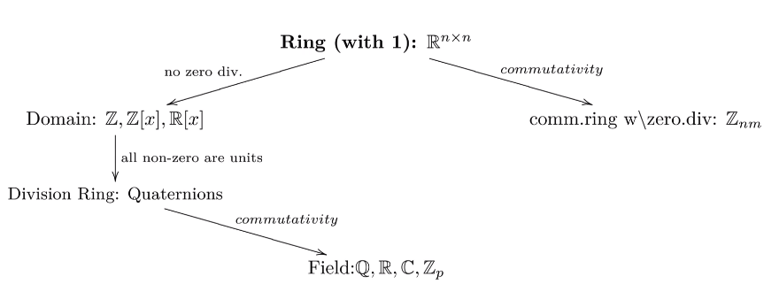
A set $R$, together with two binary operations (we’ll use addition, $+$, and multiplication, $\cdot$), is called a ring if the following conditions are satisfied:

1. $(R,+)$ is a Abelian group;
2. $(R,\cdot)$ is a semigroup;
3. the distributive laws hold; that is, for every $a$, $b$, and $c$ in $R$, we have:$a*(b+c)=a\ast b+a\ast c\qquad (a+d)\ast c=a\ast c+d\ast c.$

The smallest positive integer $n$ such that $na = 0$ for every $a$ in R (if such an $n$ exists) is called the characteristic of the ring, and we write $\text{char} R = n$.

If the multiplicative semigroup $(R, \cdot )$ is a monoid-that is, if there’s a multiplicative identity-then $R$ is called a ring with unity. The identity of the additive abelian group $(R, +)$ is usually denoted by $0$ and, in a ring with unity, the identity of the multiplicative monoid $(R, \cdot )$ is usually denoted by 1.

If the operation of multiplication is commutative, then we call $R$ a commutative ring. (The term abelian is generally not used to describe a ring in which multiplication is commutative.)

If $S$ is a subset of $R$, and $S$ satisfies the ring requirements with the same operations as $R$, then we say that $(S, +, \cdot )$ is a subring of $(R, +, \cdot)$.

• ring of polynomial. The ring of polynomials with coefficients in a ring $R$ is usually denoted by $R[x_1,\cdots,x_n]$ or $R[x]$ where $x$ refer to the set of variables $\{x_1,\cdots,x_n\}$. An element $f(x)\in \mathbb{R}[x]$ can be written as a finite sum $f(x)=\sum\limits_b b_{\alpha} x^{\alpha},$
  where $\alpha=(\alpha_1,\cdots,\alpha_d)$ is a multi-index and $\alpha_i\in \mathbb{R}$.

Let $I$ be a subring of a ring $R$. If $\forall\ r\in R,x\in I$, $rx\in I$ and $xr\in I$, then $I$ is called an ideal on $R$. Every ring $R$ has at least two ideals, $\{ 0 \}$ and $R$.

Ring Homomorphisms

Let $(R, +, \times)$ and $(R’, \oplus,\otimes)$ be rings. A function $\phi: R \rightarrow R’$ is called a ring homomorphism if both of the following conditions hold for be every $a$ and $b$ in $R$:

1. $\phi(a+b)=\phi(a)\oplus\phi(b).$
2. $\phi(a\times b)=\phi(a)\otimes\phi(b).$

• The kernel of a ring homomorphism is the set $\text{ker}\phi=\{a \in R : \phi(a) = 0’\}$, where $0’ $ is the additive identity in $R’$ and is always a subring of $R$.
• The image of $R$, $\phi(R)=\{\phi(r):r\in R\}$ is a subring of $R’$.
• The image of $0$, the additive identity in $R$, must be $0’$.

Domains

A domain is a nonzero ring with unity, in which $ab = 0$ implies $a = 0$ or $b = 0$.

A commutative domain is called an integral domain.

The cancellation law holds for domains.

Fields

Let $a$ be a nonzero element of a ring $R$ with unity. If $a$ is invertible, then $a$ is called a unit. If every nonzero element in $R$ is a unit, i.e. $(R^{\ast },\cdot)$ is a group, then $R$ is called a divison ring. A division ring is a ring with exactly two ideals.

A commutative division ring is called a field. A domain where all non-zero elements are units is a field.

Every finite integral domain is a field. A finite division ring must be commutative.

The ring $\mathbb{Z}_n$ is a field if and only if $n$ is a prime.

The field has no zero divisors since a zero divisor is not invertible.

Separable Equations

A differential equation of the form $\frac{\mathrm{d} y }{\mathrm{d}x}=\frac{f(x)}{g(x)}$ is called separable because its variables can be separated. The solution to it is given by $\int g(y)\mathrm{d}y=\int f(x)\mathrm{d}x.$

Homogeneous Equations

A function of two variables, $f(x, y)$, is said to be homogeneous of degree $n$ if there is a constant $n$ such that $f(tx,ty)=t^nf(x,y)$ for all $t,x$ and $y$ for which both sides are defined. A differential equation of the form $M(x,y)\mathrm{d}x+N(x,y)\mathrm{d}y=0$ is homogeneous if $M$ and $N$ are both homogeneous functions of the same degree.

To solve this equation, let $y=xv$, $\mathrm{d}y=x\mathrm{d}v+v\mathrm{d}x$, then the equation will become separable. After solving for solution concerning $v$ and $x$, replace $v$ by $\frac{y}{x}$ and we can get the solution to the original equation.

Exact Equations

Given a function $f(x, y)$, its total differential, $\mathrm{d}f$, is defined as: $\mathrm{d}f=\frac{\partial f}{\partial x}\mathrm{d}x + \frac{\partial f}{\partial x}\mathrm{d}y.$ Then the family of curves $f(x, y) = c$ satisfies the differential equation, $\mathrm{d}f=\frac{\partial f}{\partial x}\mathrm{d}x + \frac{\partial f}{\partial x}\mathrm{d}y=0.$ So, if there exists a function $f(x, y)$ such that $M(x,y)=\frac{\partial f}{\partial x}$ and $N(x,y)=\frac{\partial f}{\partial y}$, then $M(x,y)\mathrm{d}x+N(x,y)\mathrm{d}y$ is called an exact differential and the equation $M(x,y)\mathrm{d}x+N(x,y)\mathrm{d}y=0$ is said to be an exact equation whose solution is the family $f(x,y)=c$.

If $\frac{\partial M}{\partial y}$ and $\frac{\partial N}{\partial x}$ are continuous, then the sufficient and necessary condition for the equation to be exact is that $\frac{\partial M}{\partial y}=\frac{\partial N}{\partial x}$

Nonexact Equations And Itegreating Factors

If a nonexact equation has a solution, then an integrating factor $\mu(x,y)$ is guaranteed to exist such that $\mu(x,y)M(x,y)\mathrm{d}x+\mu(x,y)N(x,y)\mathrm{d}y=0$ is an exact equation.

If $\xi(x)=\frac{M_y-N_x}{N}$ is a function of $x$ alone, then $\mu(x)=e^{\int\xi(x)\mathrm{d}x}$.

If $\phi(y)=\frac{M_y-N_x}{-M}$ is a function of $y$ alone, then $\mu(x)=e^{\int\phi(y)\mathrm{d}y}$.

First-Order Linear Equations

A first-order linear equation is defined as a differential equation of the form: $\frac{\mathrm{d}y}{\mathrm{d}x}+P(x)y=Q(x).$ The integrating factor for this equation is $\mu(x)=e^{\int P(x)\mathrm{d}x}$. Then $\frac{\mathrm{d}(\mu y)}{\mathrm{d}x}=\mu Q$. Integrating both sides gives the general solution $y=\frac{1}{\mu}\int \mu Q \mathrm{d}x.$

Higher-Order Linear Equations With constant Coefficients

The linear homogeneous differential equation of the
$n$th order with constant coefficients can be written as $y^{(n)}+ a_1 y^{(n-1)}+\cdots + a_n y=0,$
where $a_1,\ldots,a_n\in \mathbb{C}$. For each differential operator with constant coefficients, we can introduce the characteristic polynomial $L(\lambda)=\lambda^n+a_1\lambda^{n-1}+\cdots+a_n.$
The algebraic equation $L(\lambda)=0$ is called the characteristic equation of the differential equation.

• If all roots of the characteristic equation are real and distinct, then the general solution is of the form $y=C_1e^{\lambda_1 x}+\cdots +C_ne^{\lambda_n x}$ where $\lambda_1,\ldots,\lambda_n\in \mathbb{R}$ are distinct roots and $C_1,\ldots,C_n\in\mathbb{C}$ are constants.
• If all roots of the characteristic equation are real and multiple, then the general solution is of the form $y=\sum\limits_{i=1}^m\sum\limits_{j=1}^{k_i}C_{ij}x^{j-1}e^{\lambda_i x}$
  where $\lambda_1,\ldots,\lambda_m\in \mathbb{R}$ are roots with multiplicity $k_1,\ldots,k_m$ and $\sum\limits_{i=1}^mk_i=n$, and $C_{ij}\in\mathbb{C}$ are constants.
• If all roots of the characteristic equation are complex and distinct, then the general solution is of the form $y=\sum\limits_{j=1}^{\frac{n}{2}}e^{\alpha_j x}[C_{j1}\cos(\beta_j x)+C_{j2}\sin(\beta_j x)]$ where $\alpha_j\pm i\beta_j\in \mathbb{C}$ are distinct complex roots and $C_{j1},C_{j2}\in\mathbb{C}$ are constants.
• If all roots of the characteristic equation are complex and multiple, then the general solution is of the form $y=\sum\limits_{j=1}^{\frac{n}{2}}\sum\limits_{l=1}^{k_j}e^{\alpha_j x}x^{l-1}[C_{j1}\cos(\beta_j x)+C_{j2}\sin(\beta_j x)]$ where $\alpha_j\pm i\beta_j\in \mathbb{C}$ are complex roots with multiplicity $k_j$ and $C_{j1},C_{j2}\in\mathbb{C}$ are constants.

Systems of Linear Differential Equations

In matrix form, a system of first-order linear homogeneous differential equations with constant coefficients is given by

for $\mathbf{x}(t),\mathbf{x}’(t)\in\mathbb{R}$. In the case where $\mathbf{A}$ has $n$ linearly independent eigenvectors, this differential equation has the following general solution,

where $\lambda_1, \lambda_2, \ldots, \lambda_n$ are the eigenvalues of $\mathbf{A}$; $\mathbf{u}_1, \mathbf{u}_2, \ldots, \mathbf{u}_n$ are the respective eigenvectors of $\mathbf{A}$; and $c_1, c_2, \ldots, c_n$ are constants.

Analytic Geometry Of $\mathbb{R}^3$

Vector Products

The Dot Product

The dot product is give by

where $\theta$ is the angle between $A$ and $B$.

The Cross Product

The corss product $A\times B$ is the vector that’s perpendicular by right-hand rule to the plane containing $A$ and $B$ and whose magnitude is $|A||B|\sin\theta$.

$|A\times B|$ is the area of the parallelogram formed by $A$ and $B$.

Also, we have $A\times B=\left|\begin{matrix}i & j & k\\ a_1&a_2&a_3\\ b_1&b_2&b_3\end{matrix}\right|,$
where $i,j,k$ are the standard coordinate unit basis.

The Triple Scalar Product

The triple scalar product is $(A\times B)\cdot C$. $|(A\times B)\cdot C|$ is the volume of parallelepiped formed by $A$, $B$ and $C$. Also, $(A\times B)\cdot C=\left|\begin{matrix} a_1&a_2&a_3\\ b_1&b_2&b_3\\ c_1&c_2&c_3\end{matrix}\right|.$

Geometry

Lines

The distance $d$ from a point $({ x }_{ 0 },{ y }_{ 0 })$ to the line $Ax+By=C$ is given by $d=\frac{|Ax_0+By_0-C|}{\sqrt{A^2+B^2}}.$

The nearest point to the origin in the line $Ax+By=C$ is given by $\left(\frac{AC}{A^2+B^2},\frac{BC}{A^2+B^2}\right),$ and the corresponding distance is $d=\frac{\sqrt{(AC)^2+(BC)^2}}{A^2+B^2}=\frac{|C|}{\sqrt{A^2+B^2}}.$

If we want to find the nearest point in the line to a point $(x_0,y_0)$, we can first transform to a new coordinate system by setting $x’=x-x_0$ and $y’=y-y_0$. The line becomes $Ax’+By’=C-Ax_0-By_0$. Then the nearest point in the new coordinate system is given by $\left(\frac{A(C-Ax_0-By_0)}{A^2+B^2},\frac{B(C-Ax_0-By_0)}{A^2+B^2}\right).$
By transforming it back to the original system, we have

Planes

A convinient way to represent the equation for a plane is by $\mathbf{n}\cdot (\mathbf{x} − \mathbf{p}) = 0$, where $\mathbf{p}$ is the vector to a point in the plane, and $\mathbf{n}$ is a normal vector to the plane.

The nearest point to the origin in the plane $Ax+By+Cz=D$ is given by $\left(\frac{AD}{A^2+B^2+C^2},\frac{BD}{A^2+B^2+C^2},\frac{CD}{A^2+B^2+C^2}\right),$
and the distance $d$ from the origin to this plane is given by $d=\frac{\sqrt{(AD)^2+(BD)^2+(CD)^2}}{A^2+B^2+C^2}=\frac{|D|}{\sqrt{A^2+B^2+C^2}}.$

If we want to find the nearest point in the plane to a point $(x_0,y_0)$, we can apply similar method as for a line to obtain similar results.

The Intercept of Two Planes

Two planes in $\mathbb{R}^3$ are parallel, coincide, or intersect in a line. To calculate the intercept line, we need to eliminate $x$, $y$ or $z$ to get relationship between each two of them.

The Tangent Plane To A Surface

The equation of the tangent plane to the surface $z=f(x,y)$ at $P=(x_0,y_0,z_0)$ is $z-z_0=f_x|_P\cdot (x-x_0)+f_y|_P\cdot (y-y_0).$

Cylinders

Surfaces Of Revolution

And other cases are similar by replace $x$ or $y$ by $z$.

Levle Curves And Level Surfaces

For function $z=f(x,y)$, the level curve of height $c$ is given by $f(x,y)=c$.

Coordinates

Cylindrical Coordinates

The cylindrical coordinates are given by $(r,\theta,z)$ where $r=\sqrt{x^2+y^2}$ and $\theta=\arctan\frac{y}{x}$.

Spherical Coordinates

The spherical coordinates are given by $(\rho,\phi,\theta)$ where $\rho=\sqrt{x^2+y^2+z^2}$, $\theta=\arctan\frac{y}{x}$ and $\phi=\arctan\frac{\sqrt{x^2+y^2}}{z}$.

Derivatives

Partial Derivatives

Gradients

Consider the surface $z = f(x, y)$, and let $P = (x_0, y_0)$ be a point in the domain of $f$. The gradient of $f$ is the vector $\nabla f=\left(\frac{\partial f}{\partial x},\frac{\partial f}{\partial y}\right)$.

Directional Derivatives

The rate of change of $f$ at the point $P$ in the direction of a unit vector $\mathbf{u}$, is given by $D_{\mathbf{u}}f|_P=\nabla f|_P\cdot \mathbf{u}.$

The vector $\nabla f$ points in the direction in which $f$ increases most rapidly, and the magnitude of $\nabla f$ gives the maximum rate of increase.

For a function $f (x, y, z)$, the vector $\nabla f|_P$ is perpendicular (normal) to the level curve off that contains $P$.

Similar definitions and results can be given for $\mathbb{R}^3$.

Max/Min Problems

$P_0$ is a critical point of $f(x,y)$ if $\frac{\partial f}{\partial x}\big|_{P_0}=\frac{\partial f}{\partial y}\big|_{P_0}=0.$

Let $\Delta= \text{det}(H)$.

If $\Delta>0$ and $f_{xx}(P_0)<0$, then $f$ attains a local maximum at $P_0$.

If $\Delta>0$ and $f_{xx}(P_0)>0$, then $f$ attains a local minimum at $P_0$.

If $\Delta<0$, then $f$ has a saddle point at $P_0$.

If $\Delta=0$, then no conclusion can be drawn.

Integrals

Line Integrals

Line Integrals With Respect To Arc Length

Curve

Consider a function $f(x,y)$ and a curve $C$ in the $xy$-plane. A curve given parametrically by the vector equation $\mathbf{r}=r(t)=(x(t),y(t))$ is said to be smooth, if $r’(t)$ is continuous and nonzero. And it is piecewise smooth if it is composed of a finite number of smooth curves joined at consecutive endpoints.

Line Integrals In $\mathbb{R}^2$

If $C$ is an oriented, piecewise smooth curve, we partition $C$ into $n$ segments with arc length $\Delta s_i$ and choose $P_i=(x_i,y_i)$ in each segment. Then the line integral of $f$ along $C$ with respect to arc length is defined as $\int_C f\mathrm{d}s=\lim\limits_{n \rightarrow\infty}f(x_i,y_i)\Delta s_i,$
where $\mathrm{d}s=\sqrt{(\mathrm{d}x)^2+(\mathrm{d}y)^2}$.

In parametric form, $\int_C f\mathrm{d}s=\pm\int_a^b f(x(t),y(t)) \sqrt{[x'(t)]^2+[y'(t)]^2}\mathrm{d}t,$
where the sign depends on the parameter $t$. If $t$ increases in the positive direction on $C$, then we use the $+$ sign and otherwise we use the $-$ sign.

If $C$ is a closed curve, we usually use the notation $\oint_C$ to replace $\int_C$.

Line Integrals In $\mathbb{R}^3$

Analogously, we have

The Line Integrals Of A Vector Field

Vector Field

Let $D$ be a region of the plane on which a pair of continuous functions, $M(x, y)$ and $N(x, y)$, are both defined. Then the function $\mathbf{F}=F(x,y)=(M(x,y),N(x,y))$ in $D$ is a continuous vector field on $D$.

The Line Integrals Of A Vector Field In $\mathbb{R}^2$

Let $r(t)=(x(t),y(t))$ be a parameterization of the curve $C$. Then the line integral of the vector field $F$ along $C$ is defined as: $\int_C \mathbf{F}\cdot \mathrm{d} \mathbf{r}=\int_a^b \mathbf{F}(\mathbf{r}(t))\cdot \mathbf{r}'(t)\mathrm{d}t=\int_CM\mathrm{d}x+N\mathrm{d}y.$

Fundamental Theorem

The function $F(x,y)$ is a gradient field if there is a scalar field $f$ such that $F=\nabla f$. $f$ is called a potential of $F$.

If $C$ is any piecewise smooth curve oriented from the initial point $A$ to the final point $B$, and $f$ is a continuously differentiable function defined on $C$, then: $\int_C\nabla f\cdot \mathrm{d}\mathbf{r}=f(B)-f(A).$

If $F$ is a gradient field, then $F$ is conservative, that is the integral of the vector field depends only on the initial and final points of $C$. Therefore, $\oint_C \mathbf{F}\cdot\mathrm{d}\mathbf{r}=0$ for any closed curve $C$, if and only if $F$ is a gradient field.

Double Integrals

Given a function of two variables $z=f(x,y)$ and a region $S$ in the $x$-$y$ plane, the double integral of $f(x,y)$ over $S$ is defined as $\iint_{S}f(x,y)\mathrm{d}x\mathrm{d}y= \lim\limits_{n \rightarrow\infty} \sum\limits_{i=1}^n f(x_i,y_i) (\Delta x_i)(\Delta y_i),$
which is the volume of the solid region bounded by the region $S$ and the surface $z=f(x,y)$.

Green’s Theorem

A simple closed curve is one that doesn’t cross itself between its endpoints. The positive direction of the closed curve is defined as the direction you would have to walk in order to keep the region enclosed by the curve on your _left_.

Consider a simple closed curve $C$ enclosing a region $D$, so that $C$ is the boundary of $D$. If $M(x,y
)$ and $N(x,y)$ are functions that has coontinuous partial derivatives both on $C$ and throughout $D$, then Green’s theorem says that:$\oint_CM\mathrm{d}x+N\mathrm{d}y=\iint_{D}\left(\frac{\partial N}{\partial x}-\frac{\partial M}{\partial y}\right)\mathrm{d}x\mathrm{d}y.$

It connects line integrals with double integrals in the region bounded by the line.

What is machine learning?

Definition

• Literlly, “machine” denotes “programming computer” and “learning” denotes “learn from data”.
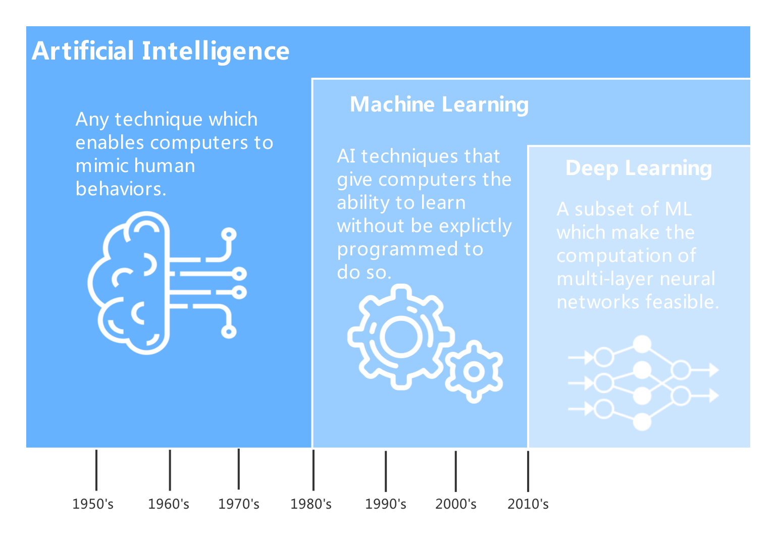
• In a general sense, machine learning means that the computer can learn some ability without explicitly programming.
• From the perspective of engineering, given some task $T$, corresponding experience (training data) $E$ and performance measurement $P$, machine learning hopes to learn from $E$ so that the performance $P$ on task $T$ can be improved.

Machine learning is a interdisciplinary field, which relates to computer science, statistics, mathematics and so on.

Basic element

• Data. Every insatcne is called sample. The set of training and testing data is called training set and testing set, respectively. Since for some algorithms, parameters are required to be tuned, we need to split a subset from the training set, which is called evaluation set and used for determining how good or bad the parameters are.
• Model. It can be viewed as a function $f$. Given an input $x$, one can get an output $y$. The model may rely on some changeable parameters $\theta$. The process of learning is to update $\theta$.
• Performance measurement. It is used to evalute the performance of the model. We can use utility function, fitness function to evaluate how good a model is. And we can also use the cost function to evaluate how bad a model is.

Procedure

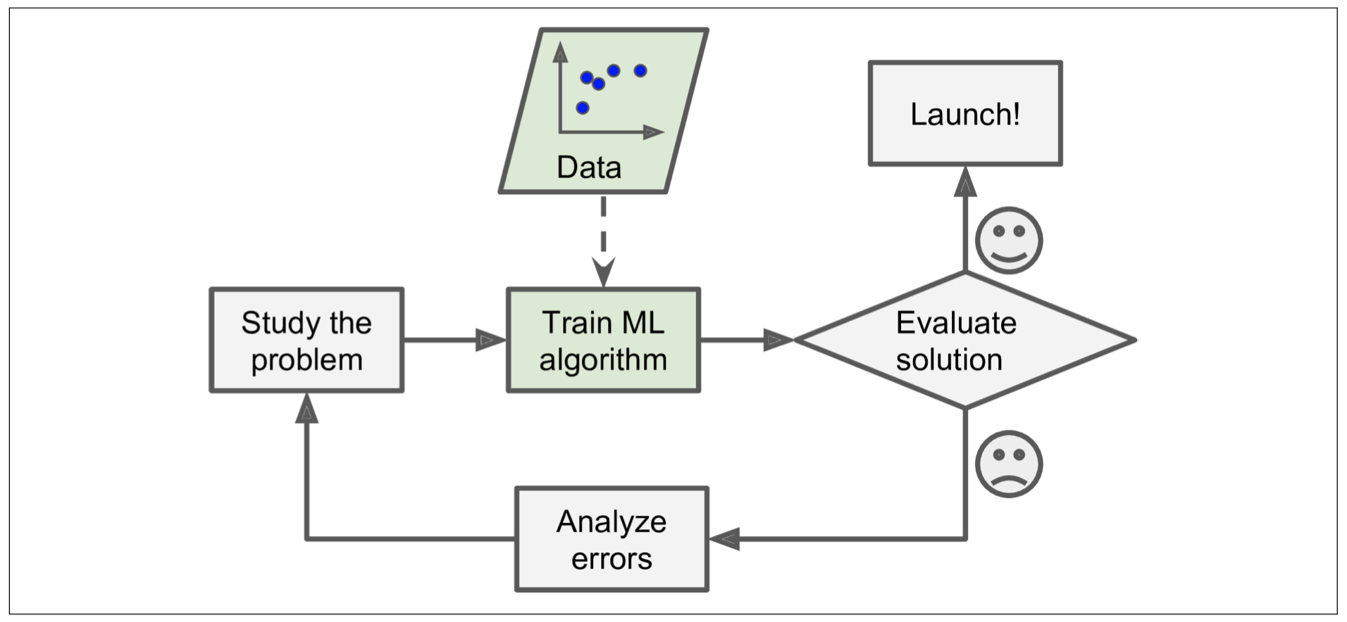
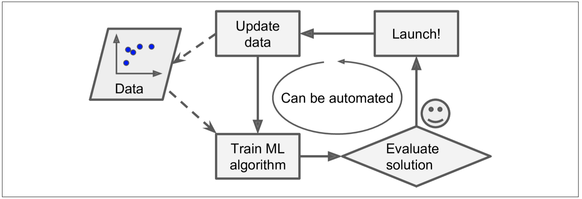
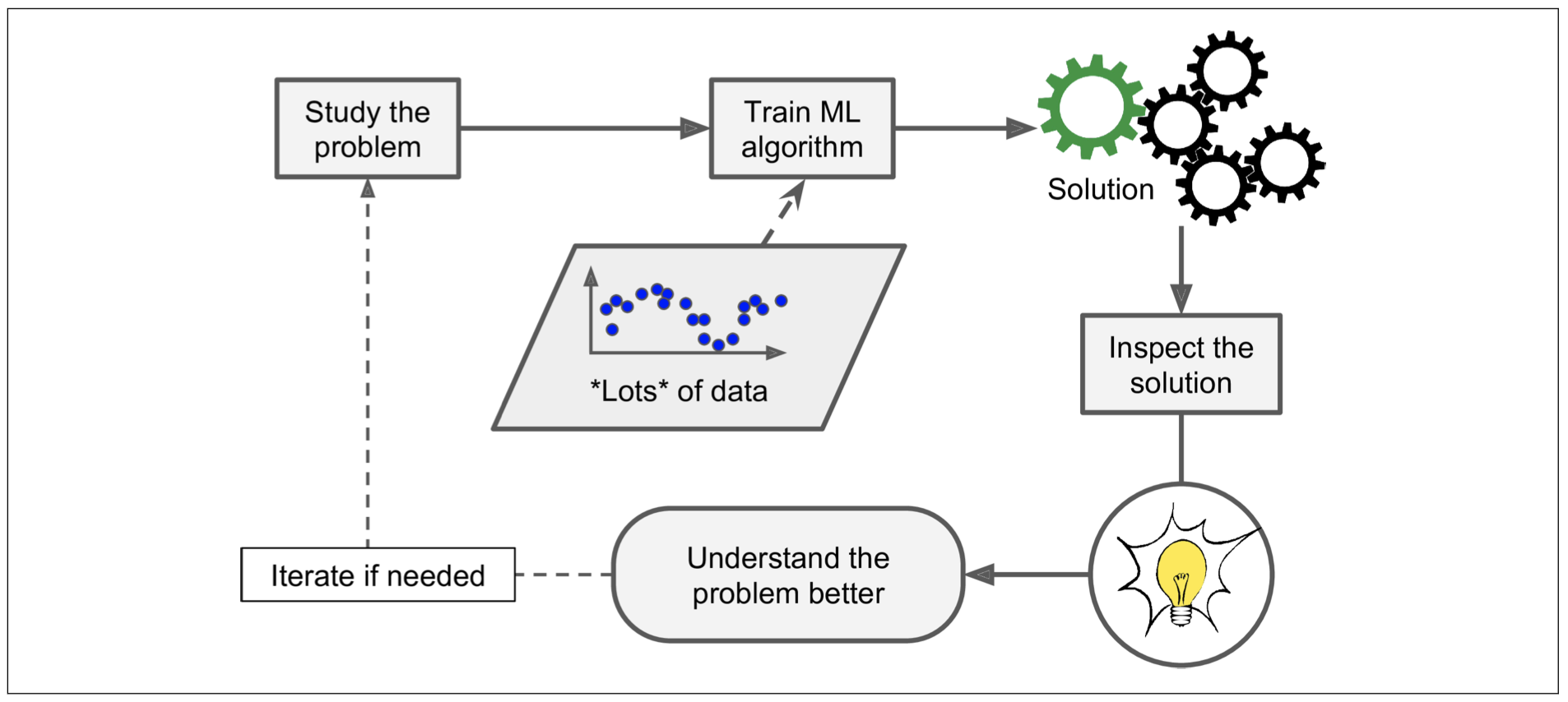
• To study data;
• To select a model;
• To train the model on the training set;
• To make a(n) prediction/inference on new data.

Why use machine learnig?

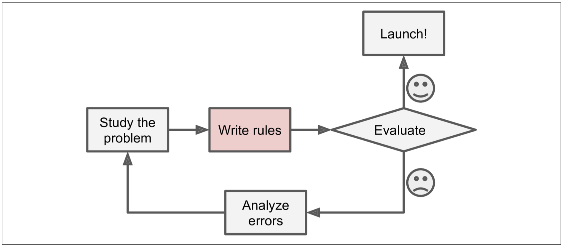
• To do work that requires a lot of hand-tuning or long lists of rules;

• To adpat to change of environment/data;

• To solve problems that is difficult for human;
• To learning unkonwn rules (data mining)

Types of machine learning

There are many categories for machine learning algorithms. Generally, we can classify them from the following perspectives.

Training data

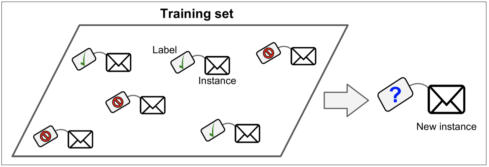
Supervised learning.

In supervised learning, each training sample $x\in \mathscr{X}$ has a label $y\in\mathscr{Y}$.

• Classification. The label set $\mathscr{Y}$ consists of finite elements, such as $\{0,1\}$, $\{\text{Yes}, \text{No}\}$ and so on. The classification task is to determine which class is for a given sample.

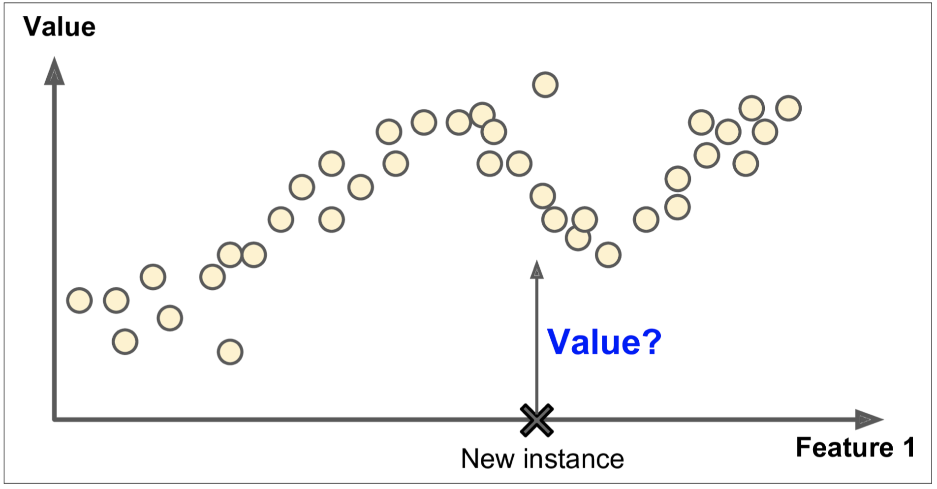
• Regression. The label set $\mathscr{Y}$ consists of an interval or even more complex elements, such as $[0,1]$. The regression task is to find a suitable map from $\mathscr{X}$ to $\mathscr{Y}$.

• Ranking. The samples are splitted into different group, and the label set can either be discrete or continuous. This is a special task and commonly used in recommended systems. It aims to give ranks of samples in a group.

Some common supervised learning algorithms are given below:

• k-Nearest Neighbors
• Linear Regression
• Logistic Regression
• Support Vector Machines (SVMs)
• Decision Trees and Random Forests
• Neural networks

Unsupervised learning.

• Clustering
  • K-Means
  • DBSCAN
  • Hierarchical Cluster Analysis (HCA)
• Anomaly detection and novelty detection
  • One-class SVM
  • Isolation Forest
• Visualization and dimensionality reduction
  • Principal Component Analysis (PCA)
  • Kernel PCA
  • Locally-Linear Embedding (LLE)
  • t-distributed Stochastic Neighbor Embedding (t-SNE)
• Association rule learning
  • Apriori
  • Eclat

Semisupervised learning.

Reinforcement learning.

Learning

• Offline learning/batch learning.
• Online learning.

Generalizing

• Instance-based learning.
• Model-based learning.

Main challenges of machine learning

Data

• Lack of training data;
• Lack of representitive of training data;
• Poor quaility of training data;
• Irrelevant features.

Model

• Overfitting of models on training data;
• Underfitting of models on training data.

References

1. Hands-on Machine Learning with Scikit-Learn, Keras, and TensorFlow, 2nd Edition

Definition

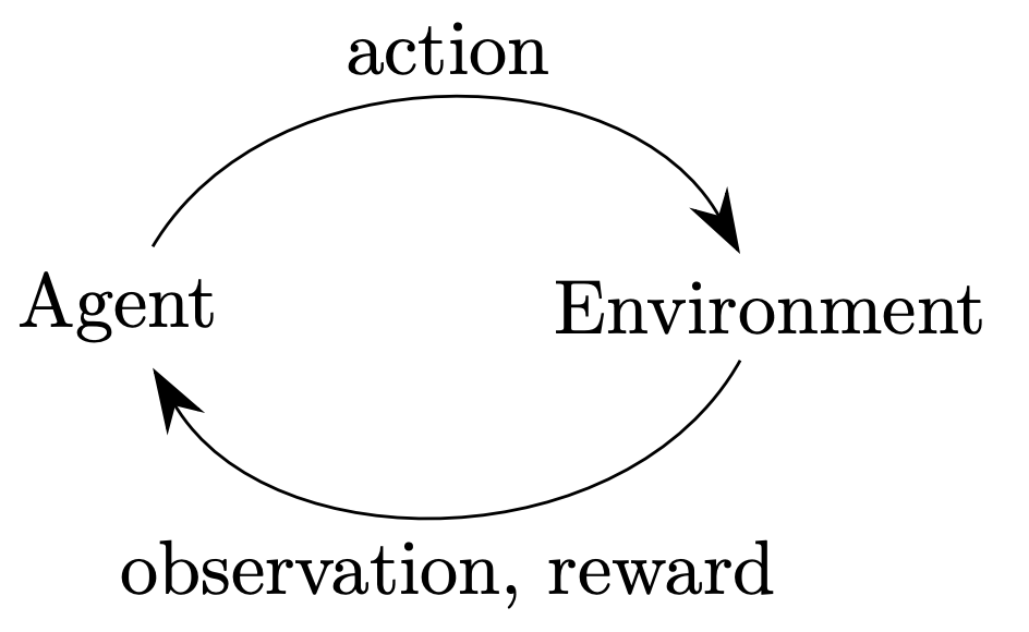
A discrete-time partially observable Markov decision process (POMDP) models the relationship between an agent and its environment. Formally, a POMDP is a 7-tuple $(S,A,T,R,\Omega,O,\gamma)$, where

• $S$ is a set of states;
• $A$ is a set of actions;
• $T$ is a set of conditional transition probabilities between states;
• $R: S \times A \to \mathbb{R}$ is the reward function;
• $\Omega$ is a set of observations,
• $O$ is a set of conditional observation probabilities;
• $\gamma \in [0, 1]$ is the discount factor.

At each time period, the environment is in some state $s\in S$. The agent takes an action $a\in A$, which causes the environment to transition to state $s’$ with probability $T(s’|s,a)$. At the same time, the agent receives an observation $o\in \Omega$ which depends on the new state of the environment, $s’$, and on the just taken action, $a$, with probability $O(o|s’,a)$. Finally, the agent receives a reward $r$ equal to $R(s, a)$. Then the process repeats. The goal is for the agent to choose actions at each time step that maximize its expected future discounted reward: $\mathbb{E}\left[\sum_{t=0}^{\infty}{\gamma}^tr_t\right]$, where $r_t$ is the reward earned at time $t$. The discount factor $\gamma$ determines how much immediate rewards are favored over more distant rewards.

When $\gamma =0$ the agent only cares about which action will yield the largest expected immediate reward; when $\gamma =1$ the agent cares about maximizing the expected sum of future rewards.

Belief MDP

The belief $b(s)$ of the agent is a function describing the probability of being in state $s$ at one moment. After having taken the action $a$ and observing $o$, an agent needs to update its belief in the state the environment may (or not) be in. Since the state is Markovian (by assumption), maintaining a belief over the states solely requires knowledge of the previous belief state, the action taken, and the current observation. The operation is denoted $b’ = \tau(b,a,o)$. Below we describe how this belief update is computed.

After reaching $s’$, the agent observes $o\in \Omega$ with probability $O(o\mid s’,a)$. Let $b$ be a probability distribution over the state space $S$. $b(s)$ denotes the probability that the environment is in state $s$. Given $b(s)$, then after taking action $a$ and observing $o$,

where $\eta =\frac{1}{\mathbb{P}(o\mid b,a)}$ is a normalizing constant with $\mathbb{P}(o\mid b,a)=\sum _{s’\in S}O(o\mid s’,a)\sum_{s\in S}T(s’\mid s,a)b(s)$.

A Markovian belief state allows a POMDP to be formulated as a Markov decision process where every belief is a state. The resulting belief MDP will thus be defined on a continuous state space (even if the “originating” POMDP has a finite number of states: there are infinite belief states (in $B$) because there are an infinite number of mixtures of the originating states (of $S$)), since there are infinite beliefs for any given POMDP.

Formally, the belief MDP is defined as a tuple $(B,A,\tau,r,\gamma)$ where

• $B$ is the set of belief states over the POMDP states;
• $A$ is the same finite set of action as for the original POMDP;
• $\tau$ is the belief state transition function;
• $r:B \times A \to \mathbb{R}$ is the reward function on belief states;
• $\gamma$ is the discount factor equal to the $\gamma$ in the original POMDP.

Of these, $\tau$ and $r$ need to be derived from the original POMDP. $\tau$ is

where $\mathbb{P}(o|a,b)$ is the value derived in the previous section and

The belief MDP reward function ($r$) is the expected reward from the POMDP reward function over the belief state distribution:

The belief MDP is not partially observable anymore, since at any given time the agent knows its belief, and by extension the state of the belief MDP.

Policy And Value Function

Unlike the “originating” POMDP (where each action is available from only one state), in the corresponding Belief MDP all belief states allow all actions, since you (almost) always have some probability of believing you are in any (originating) state. As such, $\pi$ specifies an action $a=\pi(b)$ for any belief $b$.

Here it is assumed the objective is to maximize the expected total discounted reward over an infinite horizon. When $R$ defines a cost, the objective becomes the minimization of the expected cost.

The expected reward for policy $\pi$ starting from belief $b_{0}$ is defined as

where $\gamma<1$ is the discount factor. The optimal policy $\pi^\ast$ is obtained by optimizing the long-term reward.

where $b_{0}$ is the initial belief.

The optimal policy, denoted by $\pi^\ast$, yields the highest expected reward value for each belief state, compactly represented by the optimal value function $V^{\ast}$. This value function is solution to the Bellman optimality equation:

For finite-horizon POMDPs, the optimal value function is piecewise-linear and convex. It can be represented as a finite set of vectors. In the infinite-horizon formulation, a finite vector set can approximate $V^{\ast}$ arbitrarily closely, whose shape remains convex. Value iteration applies dynamic programming update to gradually improve on the value until convergence to an $\epsilon$-optimal value function, and preserves its piecewise linearity and convexity. By improving the value, the policy is implicitly improved. Another dynamic programming technique called policy iteration explicitly represents and improves the policy instead. These are the same as value iteration and policy iteration MDP.

Introduction

Reinforcement learning is a computational goal-directed approach to learning from interaction with environment.

• trial-and-error search
• delayed reward

We can use ideas from dynamical systems theory to formulate a reinforcement learning problem, specifically, as the optimal control of incompletely-known Markov decision processes. A learning agent must be able to sense the state of its environment to some extent and must be able to take actions that affect the state. The agent also must have a goal or goals relating to the state of the environment.

One of the challenges that arise in reinforcement learning, and not in other kinds of learning, is the trade-off between exploration and exploitation. The agent has to exploit what it has already experienced in order to obtain reward, but it also has to explore in order to make better action selections in the future.

Methods based on general principles, such as search or learning, were characterized as “weak methods,” whereas those based on specific knowledge were called “strong methods.”

Taxonomy

In reinforcement learning, we have two orthogonal choices: what kind of objective to optimize (involving a policy, value function, or dynamics model), and what kind of function approximators to use.

First, we have two kinds of algorithms:

• Model-based RL algorithms: based on dynamics model that tends to predict the next state and the reward at the next step;
• Model-free RL algorithms: not based on a dynamics model.

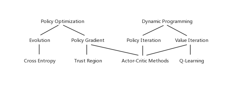
Then, for model-free RL algorithms, the figure below shows a taxonomy:

Policy optimization methods are centered around the policy, the function that maps the agent’s state to its next action. These methods view reinforcement learning as a numerical optimization problem where we optimize the expected reward with respect to the policy’s parameters. There are two ways to optimize a policy.

1. Derivative free optimization (DFO) algorithms, including evolutionary algorithms, like genetic programming, simulated annealing, etc.;
2. Policy gradient methods.

Approximate dynamic programming (ADP) focus on learning value functions, which predict how much reward the agent is going to receive.

Finally, there are actor-critic methods that combine elements from both policy optimization and dynamic programming. These methods optimize a policy, but they use value functions to speed up this optimization, and often use ideas from approximate dynamic programming to fit the value functions.

Elements of Reinforcement Learning

• a policy;
• a reward signal;
• a value function;
• (optionally) a model of the environment.

Markov Decision Process

A Markov decision process is a $5$-tuple $(S,A,P_{\cdot}(\cdot,\cdot),R_{\cdot}(\cdot,\cdot),\gamma)$, where

• $S$ is a finite set of states.

• $A$ is a finite set of actions (alternatively, $A(s)$ is the finite set of actions available from state $s$).

• $R_{a}(s,s’)$ is the immediate reward (or expected immediate reward) received after transitioning from state $s$ to state $s’$, due to $a$. It can also be like $R(s)$ or $R(s,a)$.

• $P_a(s,s’)=P(s_{t+1}=s’|s_t=s,a_t=a)$ is the probability that action $a$ in state $s$ at time $t$ will lead to state $s’$ at time $t+1$.

• $\gamma\in[0,1]$ is a discount factor, which represents the difference in importance between future rewards and present rewards.

The solution to the MDP is the policy $\pi(s)\rightarrow a$, which maximizes the long-term expected reward. In reinforcement learning domains, we simply assume the policy is deterministic and history-independent.

Total Reward

$V(s)$, the state value function, is the total discounted reward from time-step $t$,

We can show that

Policies

The long term and delayed reward is given by

which is not equal to the immediate reward $R(s)$.

From Bellman Equation, the value function can be decomposed into two parts:immediate reward $R(s)$ and discounted value of successor state $\gamma V(S_{t+1})$.

Similar result holds for $V^{\pi}(s)$.

Policy-Iterated RL

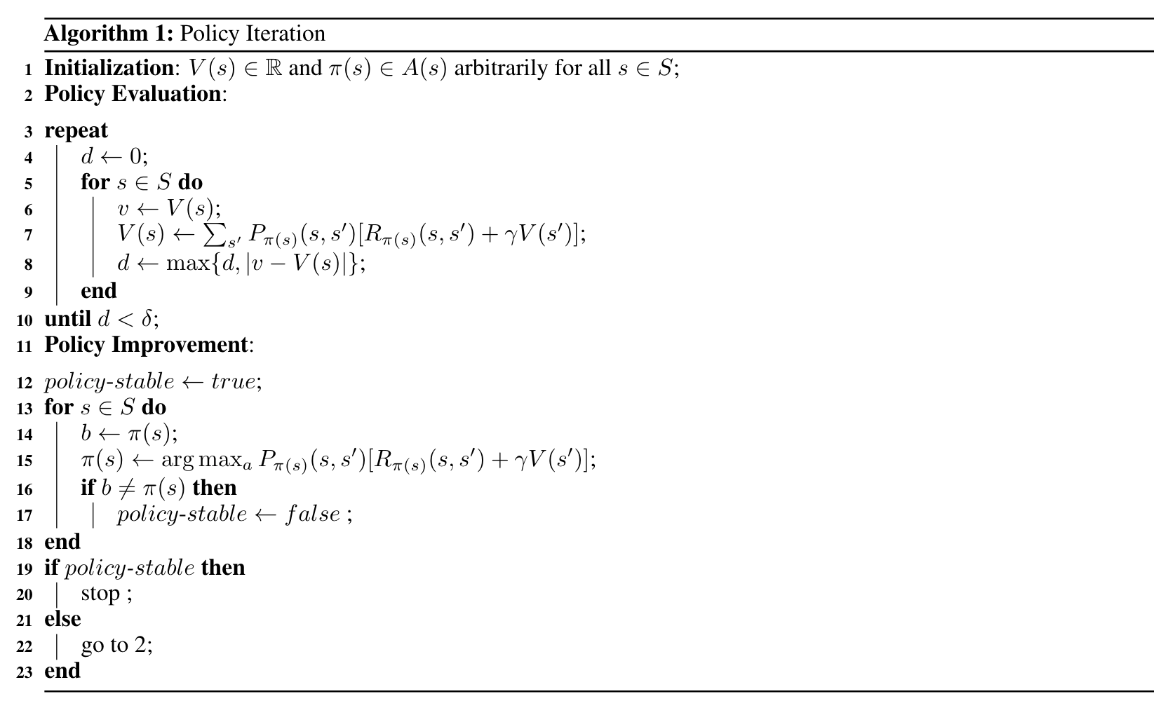
Policy iteration tries to evaluate and improve the policy in turn. Once a policy $\pi$ has been improved by using $V^{\pi}$ to yield a better policy $\pi’$, we can then compute $V^{\pi’}$ and improve it again to yield an even better policy. We can thus obtain a sequence of monotonically improving policies and value functions: $\pi_0\xrightarrow{E}V^{\pi_0}\xrightarrow{I}\pi_1\xrightarrow{E}\cdots \xrightarrow{I}V^{\pi^{\ast}}\xrightarrow{E}V^{\ast}$
where $\xrightarrow{E}$ denotes a policy evaluation and $\xrightarrow{I}$ denotes a policy improvement. Each policy is guaranteed to be a strict improvement over the previous one (unless it is already optimal). Because a finite MDP has only a finite number of policies, this process must converge to an optimal policy and optimal value function in a finite number of iterations.

Value-Iterated RL

One drawback to policy iteration is that each of its iterations involves policy evaluation, which may itself be a protracted iterative computation requiring multiple sweeps through the state set. If policy evaluation is done iteratively, then convergence exactly to occurs only in the limit.

In fact, the policy evaluation step of policy iteration can be truncated in several ways without losing the convergence guarantees of policy iteration. One important special case is when policy evaluation is stopped after just one sweep (one backup of each state). This algorithm is called value iteration. It can be written as a particularly simple backup operation that combines the policy improvement and truncated policy evaluation steps:

for all $s\in S$. For arbitrary $V_0$, the sequence $\{V_k\}$ can be shown to converge to $V^\ast$ under the $V^\ast$.

Code Example

1
2
3

import numpy as np
import gym
from gym import wrappers

Policy-Iterated RL

1
2
3
4
5
6
7
8
9
10
11
12
13
14
15
16
17
18
19
20
21
22
23
24
25
26
27
28
29
30
31
32
33
34
35
36
37
38
39
40
41
42
43
44
45

def policy_evaluation(env, policy, gamma=1.0):
    """ Iteratively evaluate the value-function under policy.
    Alternatively, we could formulate a set of linear equations in iterms of v[s] 
    and solve them to find the value function.
    """
    v = np.zeros(env.nS)
    eps = 1e-10
    while True:
        prev_v = np.copy(v)
        for s in range(env.nS):
            policy_a = policy[s]
            v[s] = sum([p * (r + gamma * prev_v[s_]) for p, s_, r, _ in env.P[s][policy_a]])
        if (np.sum((np.fabs(prev_v - v))) <= eps):
            # value converged
            break
    return v

def policy_improvement(v, gamma = 1.0):
    """ Extract the policy given a value-function """
    policy = np.zeros(env.nS)
    for s in range(env.nS):
        q_sa = np.zeros(env.nA)
        for a in range(env.nA):
            q_sa[a] = sum([p * (r + gamma * v[s_]) for p, s_, r, _ in  env.P[s][a]])
        policy[s] = np.argmax(q_sa)
    return policy

def policy_iteration(env, gamma = 1.0):
    """ Policy-Iteration algorithm """
    # initialize a random policy
    policy = np.random.choice(env.nA, size=(env.nS))
    # parameter
    max_iterations = 200000
    gamma = 1.0
    # run iterations
    for i in range(max_iterations):
        # calculate the value given the old policy
        old_policy_v = policy_evaluation(env, policy, gamma)
        # find the new policy
        new_policy = policy_improvement(old_policy_v, gamma)
        if (np.all(policy == new_policy)):
            print ('Policy-Iteration converged at step %d.' %(i+1))
            break
        policy = new_policy
    return policy

Evaluation

1
2
3
4
5
6
7
8
9
10
11
12
13
14
15
16
17
18
19
20
21
22
23
24
25
26

def run_episode(env, policy, gamma = 1.0, render = False):
    """ Runs an episode and return the total reward """
    obs = env.reset()
    total_reward = 0
    step_idx = 0
    while True:
        if render:
            env.render()
        obs, reward, done , _ = env.step(int(policy[obs]))
        total_reward += (gamma ** step_idx * reward)
        step_idx += 1
        if done:
            break
    return total_reward

def evaluate_policy(env, policy, gamma = 1.0, n = 100, render = False):
    scores = [run_episode(env, policy, gamma, render) for _ in range(n)]
    return np.mean(scores)

env_name  = 'FrozenLake8x8-v0'
env = gym.make(env_name).unwrapped
optimal_policy = policy_iteration(env, gamma = 1.0)
scores = evaluate_policy(env, optimal_policy, gamma = 1.0, render = False)
print('Average scores = ', np.mean(scores))
# Policy-Iteration converged at step 13.
# Average scores =  1.0

Value-Iterated RL

1
2
3
4
5
6
7
8
9
10
11
12
13
14
15
16
17
18
19
20
21
22
23
24
25
26
27
28

def extract_policy(v, gamma = 1.0):
    """ Extract the policy given a value-function """
    policy = np.zeros(env.nS)
    for s in range(env.nS):
        q_sa = np.zeros(env.action_space.n)
        for a in range(env.action_space.n):
            for next_sr in env.P[s][a]:
                # next_sr is a tuple of (probability, next state, reward, done)
                p, s_, r, _ = next_sr
                q_sa[a] += (p * (r + gamma * v[s_]))
        policy[s] = np.argmax(q_sa)
    return policy


def value_iteration(env, gamma = 1.0):
    """ Value-iteration algorithm """
    v = np.zeros(env.nS)  # initialize value-function
    max_iterations = 100000
    eps = 1e-20
    for i in range(max_iterations):
        prev_v = np.copy(v)
        for s in range(env.nS):
            q_sa = [sum([p*(r + prev_v[s_]) for p, s_, r, _ in env.P[s][a]]) for a in range(env.nA)]
            v[s] = max(q_sa)
        if (np.sum(np.fabs(prev_v - v)) <= eps):
            print ('Value-iteration converged at iteration# %d.' %(i+1))
            break
    return v

Evaluation

1
2
3
4
5
6
7
8
9
10
11
12
13
14
15
16
17
18
19
20
21
22
23
24
25
26
27
28
29
30
31
32
33
34
35
36
37
38
39
40
41
42
43
44
45

def run_episode(env, policy, gamma = 1.0, render = False):
    """ Evaluates policy by using it to run an episode and finding its
    total reward.
    args:
    env: gym environment.
    policy: the policy to be used.
    gamma: discount factor.
    render: boolean to turn rendering on/off.
    returns:
    total reward: real value of the total reward recieved by agent under policy.
    """
    obs = env.reset()
    total_reward = 0
    step_idx = 0
    while True:
        if render:
            env.render()
        obs, reward, done , _ = env.step(int(policy[obs]))
        total_reward += (gamma ** step_idx * reward)
        step_idx += 1
        if done:
            break
    return total_reward


def evaluate_policy(env, policy, gamma = 1.0,  n = 100):
    """ Evaluates a policy by running it n times.
    returns:
    average total reward
    """
    scores = [
            run_episode(env, policy, gamma = gamma, render = False)
            for _ in range(n)]
    return np.mean(scores)

env_name  = 'FrozenLake8x8-v0'
gamma = 1.0
env = gym.make(env_name).unwrapped
optimal_v = value_iteration(env, gamma);
policy = extract_policy(optimal_v, gamma)
policy_score = evaluate_policy(env, policy, gamma, n=1000)
print('Policy average score = ', policy_score)

# Value-iteration converged at iteration# 2357.
# Policy average score =  1.0

References

1. Policy Iteration

Introduction

Q-leaning is a model-free (no need to build a model of environment) reinforcement learning method. The goal of Q-leaning is to learn a policy, which can be used to guide a agent to take corresponding action in different states. For any finite Markov Decision Process, Q-learning can find the optimal policy that miximizes the expected total reward.

Preliminaries

Reinforcement learning includes a agent, a state set $S$ and an action set $A$. When the state $s_t\in S$ is observed, the agent will choose an action $a_t\in A$. Then it will get a reward $r_t$ and goes to the next state $s_{t+1}$.

Our goal is to maximize the future total reward, i.e., the expection of total reward given the current state. In practice, we usually use weighted sum, e.g., discount criterion to compute the expected total reward.

Q-learning is used to learn a function $Q:S\times A\mapsto \mathbb{R}$. At any state $s_t$, the agent can choose an action $a_t$ such that $Q(s_t,a_t)$ is maximized。

Algorithm

To use Q-learning, wehave to find a way to learn the $Q$ function. The simplest way is to maintain a table with size $|S|\times |A|$, and use value iteration to update the Q-table. The update rule is given by

whick requires $s_t$, $r_t$ and $s_{t+1}$ at each update step.

Code

1
2
3
4
5
6
7
8
9
10
11
12
13
14
15
16
17
18
19
20
21
22
23
24
25
26
27
28
29
30
31
32
33
34
35
36
37

import gym
import numpy as np 
# 1. Load Environment and Q-table structure
env = gym.make('FrozenLake8x8-v0')
Q = np.zeros([env.observation_space.n,env.action_space.n])
# env.obeservation.n, env.action_space.n gives number of states and action in env loaded
	
# 2. Parameters of Q-leanring
eta = .628
gma = .9
epis = 100
rev_list = [] # reward per episode calculate
	
# 3. Q-learning Algorithm
for i in range(epis):
    # Reset environment
    s = env.reset()
    rAll = 0
    d = False
    j = 0
    
    # The Q-Table learning algorithm
    while j < 99:
        env.render()
        j+=1
        # Choose action from Q table
        a = np.argmax(Q[s,:] + np.random.randn(1,env.action_space.n)*(1./(i+1)))
        # Get new state & reward from environment
        s1,r,d,_ = env.step(a)
        # Update Q-Table with new knowledge
        Q[s,a] = Q[s,a] + eta*(r + gma*np.max(Q[s1,:]) - Q[s,a])
        rAll += r
        s = s1
        if d == True:
            break
    rev_list.append(rAll)
    env.render()

Variants

1. Deep Q-learning
2. Double Q-learning
3. Double Deep Q-learning
4. Delayed Q-learning
5. Greedly GQ